4  Vizualización de datos en R

1.Cargar el conjunto de datos iris (ya está incorporado en R)

data(iris)

data(mtcars)

head(mtcars)

                   mpg cyl disp  hp drat    wt  qsec vs am gear carb
Mazda RX4         21.0   6  160 110 3.90 2.620 16.46  0  1    4    4
Mazda RX4 Wag     21.0   6  160 110 3.90 2.875 17.02  0  1    4    4
Datsun 710        22.8   4  108  93 3.85 2.320 18.61  1  1    4    1
Hornet 4 Drive    21.4   6  258 110 3.08 3.215 19.44  1  0    3    1
Hornet Sportabout 18.7   8  360 175 3.15 3.440 17.02  0  0    3    2
Valiant           18.1   6  225 105 2.76 3.460 20.22  1  0    3    1

# Cargar paquetes necesarios para visualización

library(ggplot2)
library(ggcorrplot)
library(gridExtra)
library(grid)

# Configuración del tema para ggplot2
mi_tema <- theme_minimal() +
  theme(
    plot.title = element_text(hjust = 0.5),
    axis.text = element_text(size = 10),
    axis.title = element_text(size = 12, face = "bold")
  )

4.1 Visualización de datos univariados

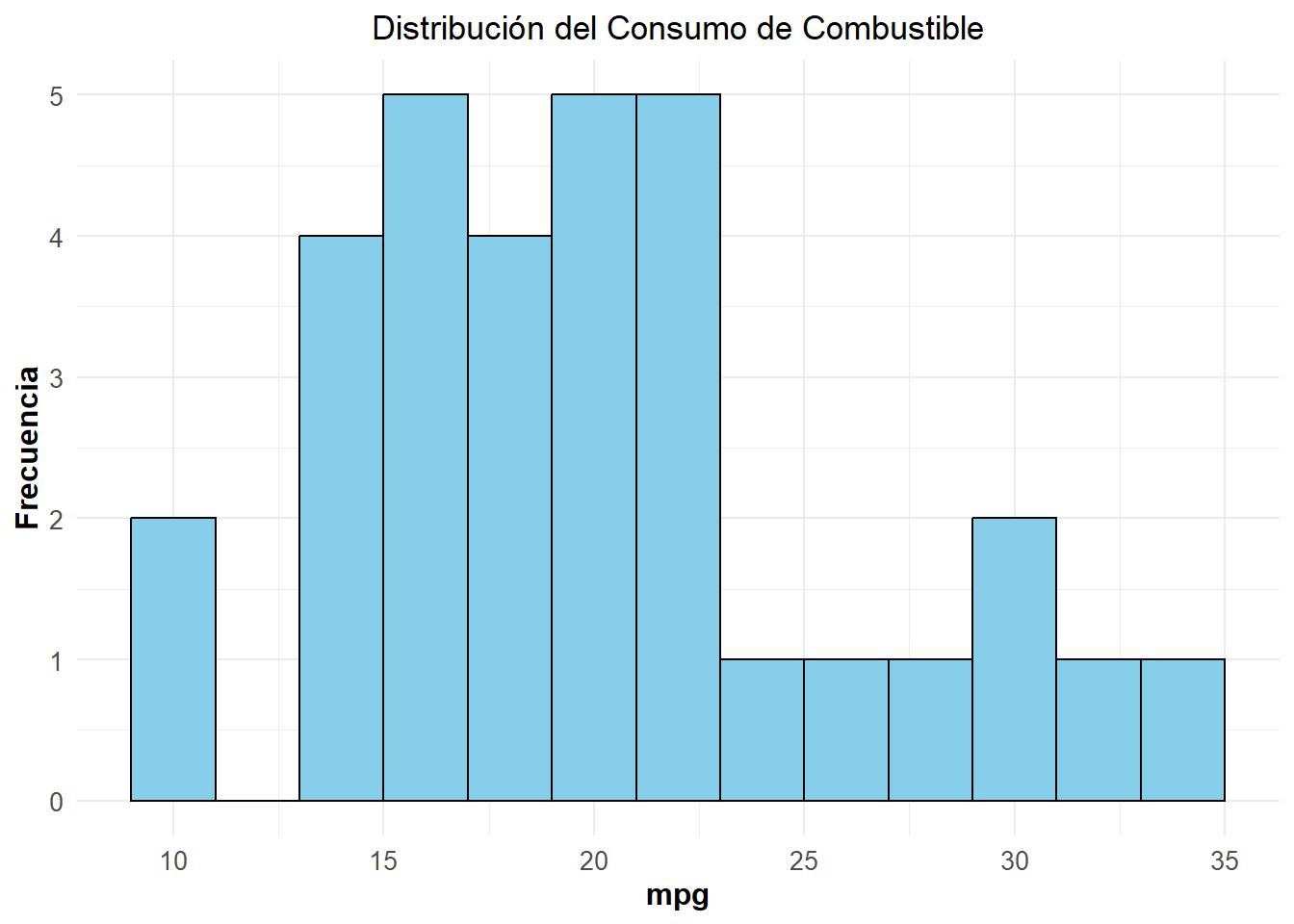
# Explorando el Consumo de Combustible (mpg)

histograma_mpg <- ggplot(mtcars, aes(x = mpg)) +
  geom_histogram(binwidth = 2, fill = "skyblue", color = "black") +
  labs(title = "Distribución del Consumo de Combustible", x = "mpg", y = "Frecuencia") +
  mi_tema

print(histograma_mpg)

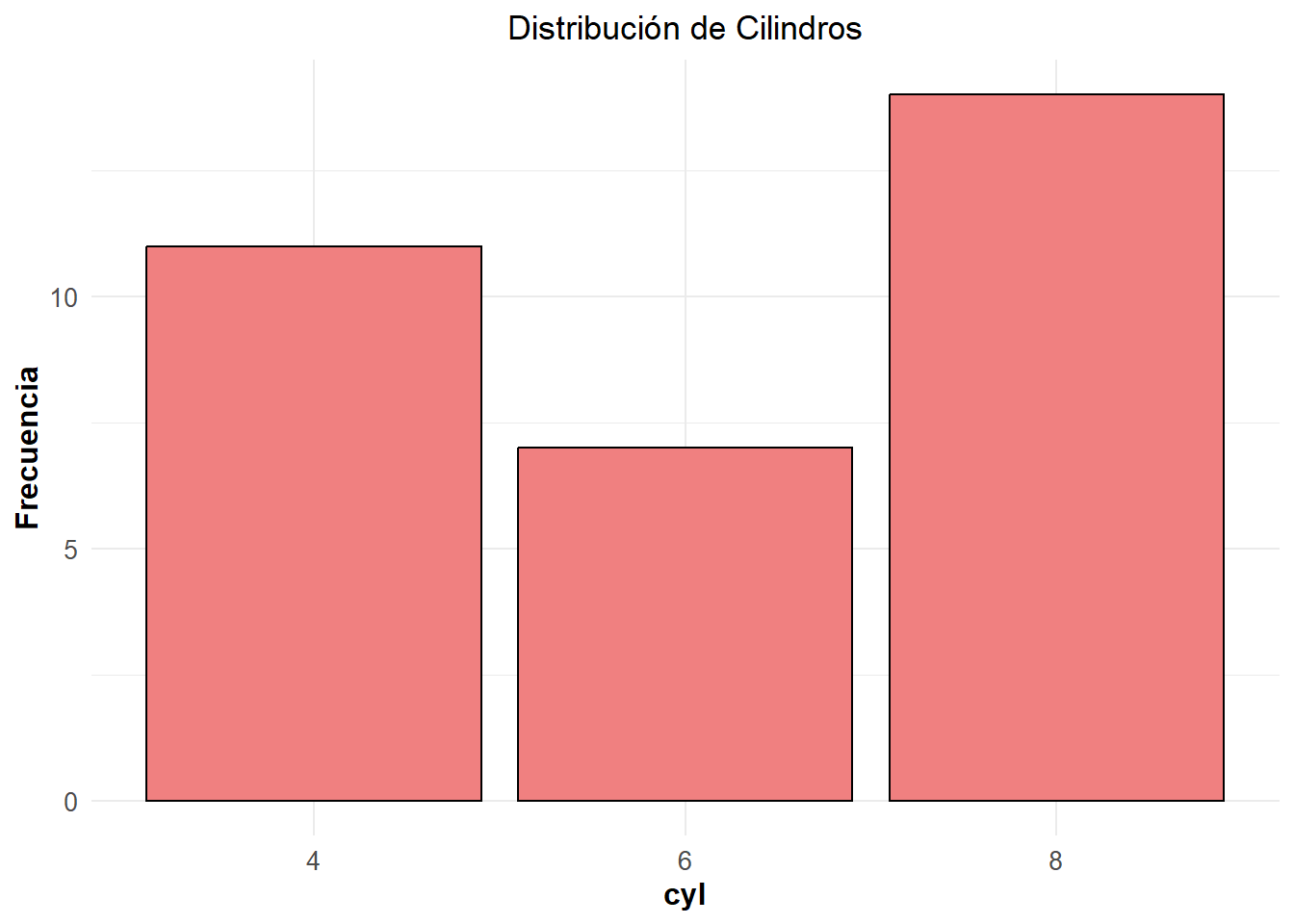
# Descubriendo la Distribución de Cilindros (cyl)
barras_cyl <- ggplot(mtcars, aes(x = factor(cyl))) +
  geom_bar(fill = "lightcoral", color = "black") +
  labs(title = "Distribución de Cilindros", x = "cyl", y = "Frecuencia") +
  mi_tema

print(barras_cyl)

4.2 Visualización de datos bivariados

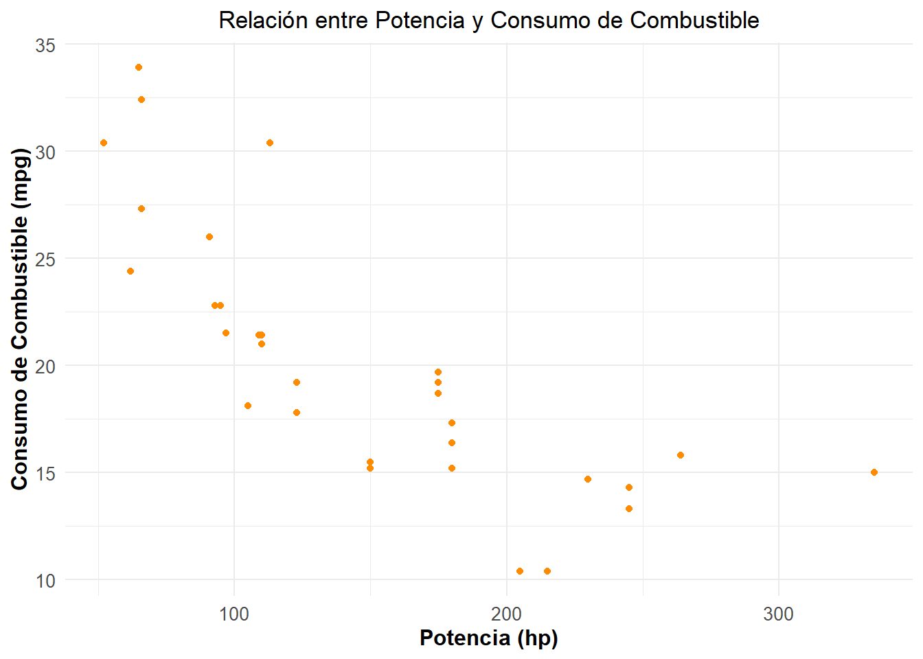
# Relación entre Potencia y Consumo de Combustible

dispersion_mpg_hp <- ggplot(mtcars, aes(x = hp, y = mpg)) +
  geom_point(color = "darkorange") +
  labs(title = "Relación entre Potencia y Consumo de Combustible", x = "Potencia (hp)", y = "Consumo de Combustible (mpg)") +
  mi_tema

print(dispersion_mpg_hp)

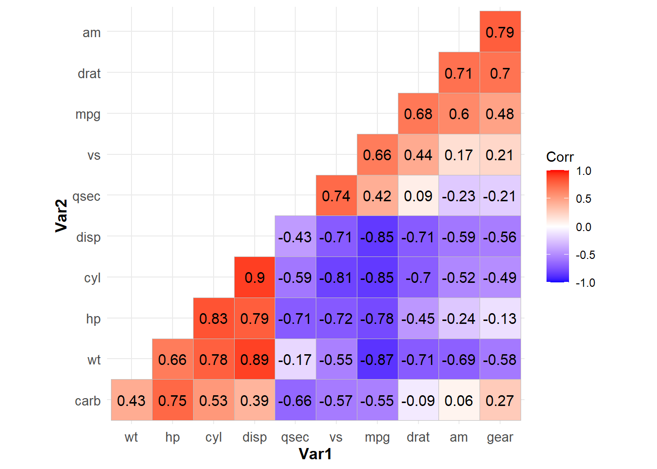
# Matriz de correlación
matriz_correlacion_mtcars <- cor(mtcars)
ggcorrplot(matriz_correlacion_mtcars, hc.order = TRUE, type = "lower", lab = TRUE) +
  mi_tema

print(matriz_correlacion_mtcars)

            mpg        cyl       disp         hp        drat         wt
mpg   1.0000000 -0.8521620 -0.8475514 -0.7761684  0.68117191 -0.8676594
cyl  -0.8521620  1.0000000  0.9020329  0.8324475 -0.69993811  0.7824958
disp -0.8475514  0.9020329  1.0000000  0.7909486 -0.71021393  0.8879799
hp   -0.7761684  0.8324475  0.7909486  1.0000000 -0.44875912  0.6587479
drat  0.6811719 -0.6999381 -0.7102139 -0.4487591  1.00000000 -0.7124406
wt   -0.8676594  0.7824958  0.8879799  0.6587479 -0.71244065  1.0000000
qsec  0.4186840 -0.5912421 -0.4336979 -0.7082234  0.09120476 -0.1747159
vs    0.6640389 -0.8108118 -0.7104159 -0.7230967  0.44027846 -0.5549157
am    0.5998324 -0.5226070 -0.5912270 -0.2432043  0.71271113 -0.6924953
gear  0.4802848 -0.4926866 -0.5555692 -0.1257043  0.69961013 -0.5832870
carb -0.5509251  0.5269883  0.3949769  0.7498125 -0.09078980  0.4276059
            qsec         vs          am       gear        carb
mpg   0.41868403  0.6640389  0.59983243  0.4802848 -0.55092507
cyl  -0.59124207 -0.8108118 -0.52260705 -0.4926866  0.52698829
disp -0.43369788 -0.7104159 -0.59122704 -0.5555692  0.39497686
hp   -0.70822339 -0.7230967 -0.24320426 -0.1257043  0.74981247
drat  0.09120476  0.4402785  0.71271113  0.6996101 -0.09078980
wt   -0.17471588 -0.5549157 -0.69249526 -0.5832870  0.42760594
qsec  1.00000000  0.7445354 -0.22986086 -0.2126822 -0.65624923
vs    0.74453544  1.0000000  0.16834512  0.2060233 -0.56960714
am   -0.22986086  0.1683451  1.00000000  0.7940588  0.05753435
gear -0.21268223  0.2060233  0.79405876  1.0000000  0.27407284
carb -0.65624923 -0.5696071  0.05753435  0.2740728  1.00000000

4.3 Visualización de datos bivariados multivariados

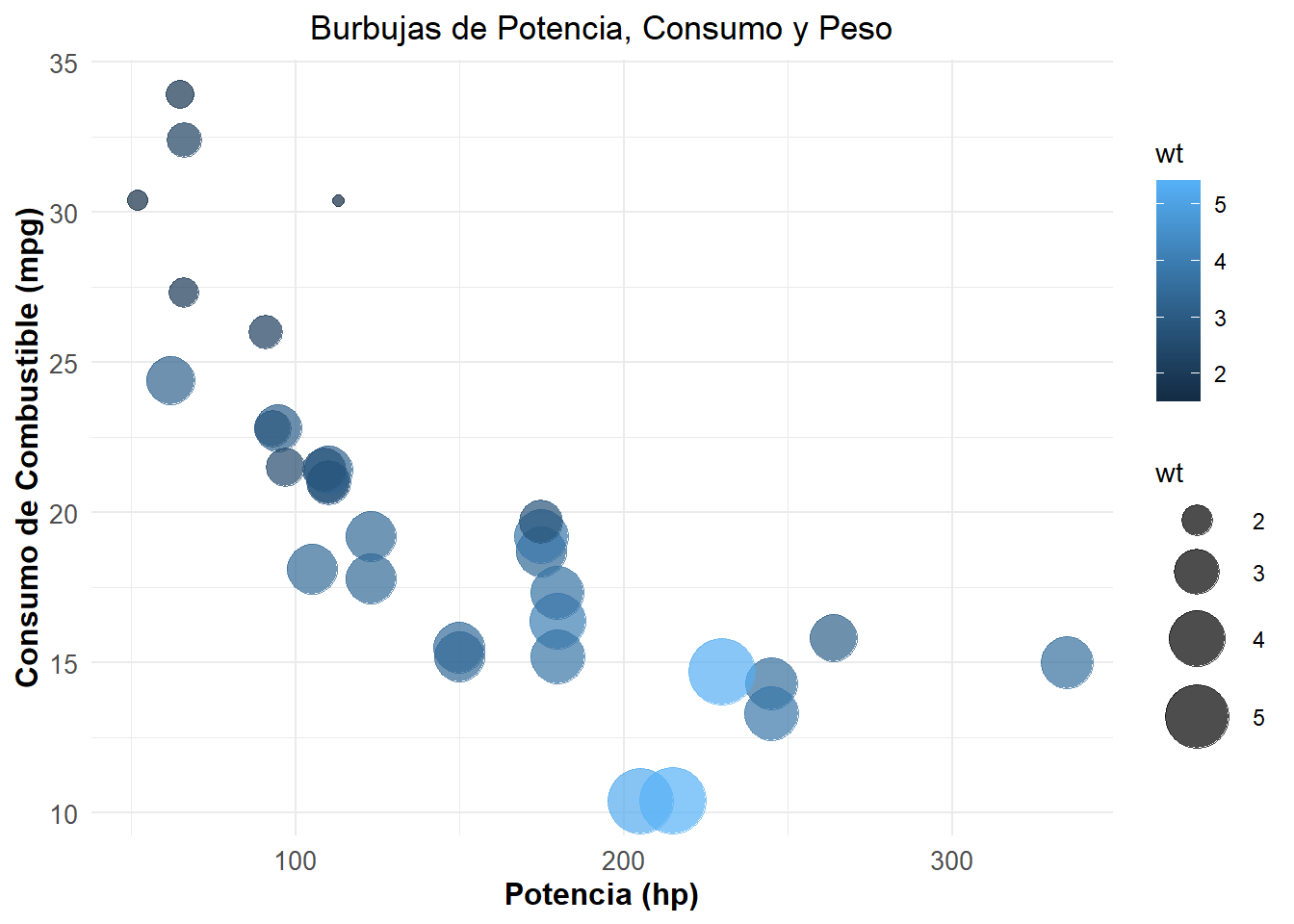
# Burbujas de Potencia, Consumo y Peso

burbujas_mpg_hp_wt <- ggplot(mtcars, aes(x = hp, y = mpg, size = wt, color = wt)) +
  geom_point(alpha = 0.7) +
  scale_size_continuous(range = c(2, 12)) +
  labs(title = "Burbujas de Potencia, Consumo y Peso", x = "Potencia (hp)", y = "Consumo de Combustible (mpg)") +
  mi_tema


print(burbujas_mpg_hp_wt)

4.4 Visualización de datos avanzados

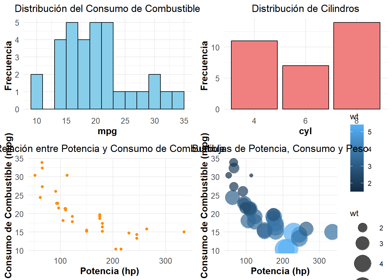
# Combinar los gráficos en una cuadrícula
grid_arrange_mtcars <- grid.arrange(
  histograma_mpg, barras_cyl, dispersion_mpg_hp, burbujas_mpg_hp_wt,
  ncol = 2
)

# Añadir título al gráfico
grid_arrange_mtcars$top <- textGrob("Exploración Visual con mtcars", gp = gpar(fontsize = 16, fontface = "bold", col = "darkblue"))

# Imprimir la cuadrícula
print(grid_arrange_mtcars)

TableGrob (2 x 2) "arrange": 4 grobs
  z     cells    name           grob
1 1 (1-1,1-1) arrange gtable[layout]
2 2 (1-1,2-2) arrange gtable[layout]
3 3 (2-2,1-1) arrange gtable[layout]
4 4 (2-2,2-2) arrange gtable[layout]